Training an Unbeatable Tic-Tac-Toe AI using Reinforcement Learning

Training the Agents

Getting Started with Ray RlLib

As mentioned before, we will be using a library called RlLib to train the neural networks that lay at the heart of our agents. RlLib is part of the larger Ray ecosystem for scaling Python applications across distributed systems. You can install RlLib with: pip install -U "ray[rllib]", which will install the Core, RlLib, and Tune libraries. See this link for more details.

Ray is a huge library, and we could spend days diving through its documentation to understand how it works. I am far from an expert on the Ray ecosystem, but I have a good-enough understanding for our purposes. At the highest level, we will:

• Use RlLib to create an algorithm config, which we will give to a tuner to be trained.
• The tuner will execute multiple copies of our algorithm simultaneously. These copies will be initialized with different hyperparameters, which affect the training progress.
• Our tuner uses a scheduler to determine if a trial should be given more time, or terminated so a new one can start.
• Based on how existing trials perform, a searcher will suggest a set of hyperparameters every time a new trial is launched.
• By intelligently searching the hyperparameter space, we make better use of our hardware resources (CPU, GPU, etc.)

Wait, What is a Hyperparameter?

If you are new to machine learning, you are probably wondering what this "hyperparameter" business is all about. While there are many great articles explaining the concept, I would be remiss if I didn't take a minute to discuss it.

When we train a neural network, we are "teaching" the network to approximate a function. This function is unknown to us and is often very complex, which is why we are using machine learning. The network approximates the function using a set of weights, which are initially random - so the approximation is bad. During training, the network uses data to update its weights in a process called gradient descent. Once the network can give us a "close-enough" approximation, training is concluded, and we have our final weights.

These weights are also called the parameters of the network. They are what we are trying to learn, and they change constantly throughout training. Hyperparameters, on the other hand, usually do not change during training. Hyperparameters affect the training process itself, such as how often we update the weights. Parameters are what we learn, hyperparameters affect how we learn it.

In our experiment, we will be tuning three hyperparameters:

• Learning Rate: The learning rate (lr) affects how quickly are weights are updated when we train on a batch of data. A large learning rate could prevent the network from converging, and a small one could make training time impractical. Read more here.
• Gamma: The discount factor for future rewards. It affects how the agent views a reward it could receive right now, versus a reward many steps into the future. Read more here
• Tie Penalty: The tie penalty is specific to our environment, and sets the reward an agent receives when the game is tied. It helps the agent understand that a tie is not as bad as a loss, but not as good as a win.

The Training Code

Alright, lets dive into the training code. It's all contained in one big function that is a lot to digest, so I will break it down and talk through each section. If you want to see the full function including the imports, take a look at the source code.

First, we define a few variables that will set limits on our training time.

• We set a maximum of 300 training iterations (epochs) for any single trial. This ensures a trial does not keep training too long and consume resources that could be spent on other trials.
• We set a total time limit of 5400 seconds, which is 1.5 hours
• We set a grace period of 15 iterations, which prevents trials from being terminated prematurely

We also initialize the ray cluster, which isn't very involved since we are using a single machine. If you had a multi-node cluster, you could use more advanced options discussed on Ray's website. At the bottom, we register our environment with Ray.

 1 def env_creator(env_config: dict):
 2     """
 3     Converts the PettingZoo Env Into an RlLib Environment
 4     """
 5     return ParallelPettingZooEnv(MultiAgentTicTacToe(env_config))
 6 
 7 
 8 experiment_name = 'My-Experiment'
 9 max_iter_individual = 300
10 max_time_total = 60 * 90
11 grace_period_iter = 15
12 ray.init()
13 register_env('tic-tac-toe', env_creator)

Now we can create our algorithm config. We will be using Proximal Policy Optimization, an on-policy algorithm you can read more about here. When creating this config object, the .##### methods can be applied in any order. The only thing that needs to be first is the PPOConfig() initializer. Let's talk through what each method configures:

• .api_stack indicates that we are using Ray's new API stack. This is a new way of interacting with the Ray ecosystem, and will be the main way to do so in the future.
• We use .reporting to alter the smoothing behavior. After each episode (tic-tac-toe game), metrics about training, learning, performance, etc. are recorded. By default, ray applies a moving average over the latest 100 episodes before reporting them to us. After observing that these metrics were very noisy, I increased the smoothing period to 1000. This reduces some of the noise and helps us focus on the overall trend.
• In .callbacks we provide a class that will report custom metrics about each tic-tac-toe game. These metrics provide clear insight to how our agents are performing.
• .environment is where we set the environment to 'tic-tac-toe' and provide configuration options. This is where our first hyperparameter, tie_penalty , appears. We tell Ray that tie_penalty can range from -1 to 1 and should be uniformly distributed.
• .multi_agent specifies that we will be training multiple policies. We provide a function to map our policies to the agents named in self.possible_agents = ['X', 'O'] from the previous section.
• .rl_module defines a module_spec for each agent. This specification tells Ray which Python class our agent will use, and if it should receive any non-default configuration. We are using a class called ActionMaskingTorchRlModule, which allows us to mask actions as previously discussed. The config dictionary sets the activation function to the Rectified Linear Unit (ReLU).
• With .training we specify the search space for our other two hyperparameters, lr and gamma. Learning rate will be sampled logarithmically so we don't under sample the lower end of our range.
• Lastly, .learners and .env_runners configure our hardware resources. We allow each trial to access 1/5 of our GPU with num_learners=0, and 2 CPUs via the env_runner config options.

 1 config = (
 2     PPOConfig()
 3     .api_stack(
 4         enable_env_runner_and_connector_v2=True,
 5         enable_rl_module_and_learner=True
 6     )
 7     .reporting(
 8         metrics_num_episodes_for_smoothing=1000
 9     )
10     .callbacks(
11         callbacks_class=Outcomes
12     )
13     .environment(
14         env='tic-tac-toe',
15         env_config={
16             'tie_penalty': tune.uniform(-1, 1),
17             'random_first': True,
18         }
19     )
20     .multi_agent(
21         policies={'pX', 'pO'},
22         policy_mapping_fn=(lambda aid, *args, **kwargs: f'p{aid}')
23     )
24     .rl_module(
25         rl_module_spec=MultiRLModuleSpec(
26             module_specs={
27                 'pX': RLModuleSpec(
28                     module_class=ActionMaskingTorchRLModule,
29                     model_config_dict={
30                         'fcnet_activation': 'relu'
31                     }
32                 ),
33                 'pO': RLModuleSpec(
34                     module_class=ActionMaskingTorchRLModule,
35                     model_config_dict={
36                         'fcnet_activation': 'relu'
37                     }
38                 )
39             }
40         )
41     )
42     .training(
43         lr=tune.loguniform(1e-5, 1e-2),
44         gamma=tune.uniform(0.80, 0.99),
45     )
46     .learners(
47         num_learners=0,
48         num_gpus_per_learner=0.2,
49     )
50     .env_runners(
51         num_env_runners=2,
52         num_cpus_per_env_runner=1,
53         num_envs_per_env_runner=1,
54     )
55 )

Next, we create a progress reporter and checkpoint configuration. The progress reporter controls how information is printed to console during the training process. I made a custom progress reporter because Ray's default was printing way too much info for me to easily discern what was happening.

The checkpoint config controls how often we save the weights of our network. If training is interrupted and crashes, we can use checkpoints to load our model and resume where we left off. We will also use a checkpoint to export our model for external use.

 1 # Create Custom Progress Reporter
 2 reporter = CustomReporter(
 3     metric_columns={
 4         'time_total_s': 'Seconds',
 5         'env_runners/Tie': 'Tie',
 6         'env_runners/WinX': 'WinX',
 7         'env_runners/WinO': 'WinO',
 8         'training_iteration': 'Iters',
 9     },
10     max_report_frequency=10,
11     metric='Tie',
12     mode='max',
13     time_col='Seconds',
14     rounding={
15         'Seconds': 0,
16         'Tie': 3,
17         'WinX': 3,
18         'WinO': 3,
19     }
20 )
21 
22 # Create Checkpoint Config
23 config_checkpoint = train.CheckpointConfig(
24     checkpoint_at_end=True,
25     num_to_keep=10,
26     checkpoint_frequency=20,
27     checkpoint_score_order='max',
28     checkpoint_score_attribute='env_runners/Tie',
29 )

Lastly, we create our tuner and call tune.fit() to begin training. In the tuner config, we specify that:

• Our key metric is env_runners/Tie, which measures how often our agents tie.
• We want to maximize this metric. Ideally our agents will tie every game, resulting in an average value of 1.
• No more than 5 trials should execute at any given time. The HyperOpt algorithm should be used to generate the hyperparameters of new trials.
• The ASHA scheduler will control termination of trials according to the variables we defined earlier
• Our sample size is -1, meaning we will continue to launch new trials until the experiment terminates.
• We have a time budget

In the tuner constructor, we provide all the objects we defined earlier. This is also where we define the stopping criteria. If a trial reaches 99% tie rate, training is considered to be complete and we stop early.

 1 # Create Tuner Config
 2 config_tuner = tune.TuneConfig(
 3     metric='env_runners/Tie',
 4     mode='max',
 5     trial_dirname_creator=trail_dirname_creator,
 6     search_alg=ConcurrencyLimiter(
 7         searcher=HyperOptSearch(),
 8         max_concurrent=5,
 9     ),
10     scheduler=ASHAScheduler(
11         time_attr="training_iterations",
12         grace_period=grace_period_iter,
13         max_t=max_iter_individual,
14     ),
15     num_samples=-1,
16     time_budget_s=max_time_total,
17 )
18 
19 # Create Tuner Object
20 os.environ['RAY_AIR_NEW_OUTPUT'] = '0'
21 tuner = tune.Tuner(
22     "PPO",
23     param_space=config,
24     run_config=train.RunConfig(
25         name=experiment_name,
26         stop={
27             'env_runners/Tie': 0.99,
28         },
29         storage_path=str(PROJECT_PATH / 'results'),
30         checkpoint_config=config_checkpoint,
31         progress_reporter=reporter,
32         verbose=1,
33     ),
34     tune_config=config_tuner
35 )
36 
37 # Start Training
38 tuner.fit()

Monitoring Training

Everything is ready to go. You crank up your GPU fan speed, take a deep breath, then click run. How do you know what's happening? After a few seconds, you should something like this in your console window:

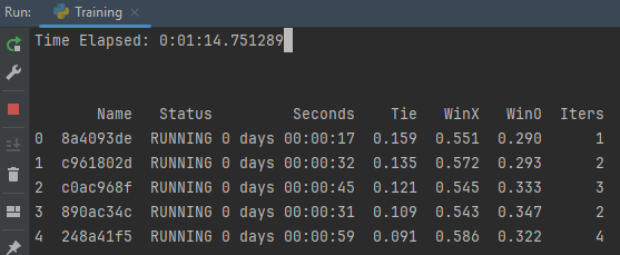
This is created by the progress reporter, which is collecting statistics, formatting them, and printing them in real-time. Trials will be sorted by their tie percentage in descending order, with RUNNING trials appearing at the top. This screenshot was taken 1 minute into training — you can see that X has a much higher win percentage than O. This makes sense, since X has the advantage of going first. As training progresses, we expect to see both WinX and WinO to decrease as Tie increases.

This table gives us insight as to how the trials rank at this moment. But what about how the trials perform over time? The answer is TensorBoard, a tool that is designed to scrap information from the result directory and create real-time graphs. While it is part of the Tensorflow ecosystem, you don't need to be using Tensorflow as your backend.

You can launch it with: tensorboard --logdir results/My-Experiment, where logdir is the folder automatically created by Ray when you start the experiment. Click the hyperlink to localhost:6006, and you should see something like this:

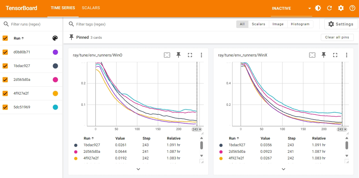
This is the Tensorboard dashboard. I won't explain everything that is going on here, but you can play around with the settings to customize the plots. Click the refresh icon in the top right (next to the gear) to update the dashboard with the latest data

Evaluating the Training Data

Tensorboard is a great tool, but you might want to do your own analysis on the training data. In order to do this, we need to extract from its log file into something more digestible. Thankfully, our work is cut-out for us since Ray already logs data in CSV format. This file is stored at results/My-Experiment/{trial_name}/progress.csv. If you open it, you will see it has many (85) columns. Let's trim this down to something more manageable and loop through all trials while we are at it.

 1 from shared.ray.result_extraction import extract_df, identify_best
 2 
 3 
 4 def create_readable_csv():
 5     """
 6     Create CSV files of key training metrics.
 7     These files can be used for plotting and comparing
 8     trials with each other.
 9     """
10     col_map = {
11         'num_env_steps_sampled_lifetime': 'EnvSteps',
12         'num_episodes_lifetime':'Episodes',
13         'training_iteration': 'Iters',
14         'time_this_iter_s': 'TimeThisIter',
15         'time_total_s': 'TimeTotal',
16         'env_runners/WinX': 'WinX',
17         'env_runners/WinO': 'WinO',
18         'env_runners/Tie': 'Tie',
19         'env_runners/episode_len_mean': 'EpisodeLengthMean',
20         'env_runners/episode_return_mean': 'EpisodeReturnMean',
21     }
22     to_keep = list(col_map.keys())
23     for trial in os.listdir('results/My-Experiment'):
24         if os.path.isdir(f'results/My-Experiment/{trial}'):
25             df = extract_df(f'results/My-Experiment/{trial}', to_keep)
26             df.rename(columns=col_map, inplace=True)
27             df = df.round(4)
28             df.to_csv(f'analysis/{trial}.csv', index=False)

Run this function, and your analysis folder should contain one CSV for each trial. But before we dig into our clean data, it might be beneficial to identify which trial yielded the best results. With a little bit of sorting and aggregation, I found that these were the top five trials from my training data:

For sake of time, let's only focus on the best trial, d0b80b71. In the following graphs, the horizontal axis represents the episode count - how many games have been played. All metrics are smoothed using a 1000 episode moving average, which we set in our training config.

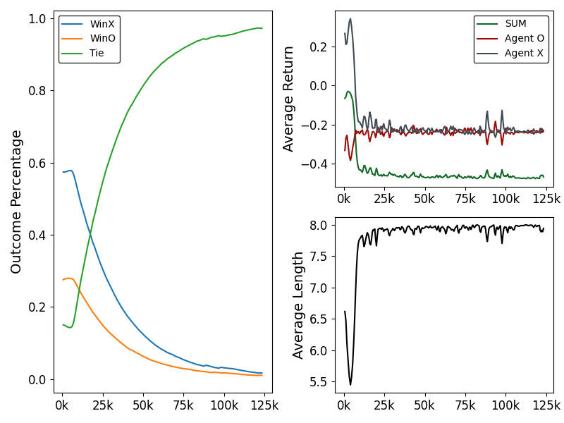
In the left graph, we see that ties dominated the outcome as training progressed. In the first few thousand episodes, tie percentage actually decreased as both agents learned basic strategies. However, it quickly increased as each agent began to prevent it's opponent from winning. This is an indication — but not a guarantee — that our agents both learned how to never lose.

On the right side, we see that the average reward (or return) for each agent quickly converged to approximately -0.2. This is not a coincidence, it corresponds to the tie_penalty for d0b80b71 which was set to -0.2389. Episode length plateaued at 8, which is one less than we would expect — a tic-tac-toe game only ties when all 9 squares are full. This is because of how ray calculates episode length and how our environment is configured. If an episode was 8 steps long, it means that 9 turns were taken by the agents.

So... does it work?

Alright. These graphs look convincing. But how do we actually know if the agents play a perfect game? After all, we stopped training when tie percentage was 97.36%, not 100%. This is partly due to how training algorithms work in reinforcement learning. When the agent is being trained, it occasionally decides deviate from a strategy it knows to produce good results in favor of trying something new. The agent does this to address the exploration-exploitation dilemma.

Under the hood, the agent samples the action probability distribution created by the policy network (as opposed to taking the argmax). Given a set of observations, it assigns probabilities to each action that represent confidence. In training, the agent chooses an action by rolling the dice. While an action that results in a mistake may be very unlikely, it is possible that the agent could select it. When using the network for inference, we always choose the action with the highest probability. This gives the agent a consistent behavior - it always responds the same way to the same input.

To decide if our agents are unbeatable, we need to export the neural networks to be used for inference. In the next section, we will export to ONNX format and evaluate how our agents perform against all possible combinations.